
The WRAPROWS function in Microsoft Excel is a useful tool for managing and organizing data. Users may use this function to organize data over numerous rows easily, break down large datasets, increase readability, and improve how information looks on the spreadsheet. This article will review the WRAPROWS function, its features, and how to use it efficiently.
What’s WRAPROWS Function In Excel?
WRAPROWS is a function that converts a one-dimensional array to a two-dimensional array. Simply put, the WRAPROWS function turns values from one row or column into an array of values from other rows. The number of rows is determined by what you provide. Because this is a freshly launched function, it is accessible to all Microsoft 365 subscribers. It is available to Microsoft 365 Basic Tier users as well.
The WRAPROWS Function Syntax
The WRAPROWS function has the following syntax.
=WRAPROWS(vector, wrap_count, [pad_with])There are three parameters to the function. Let’s break through each function parameter.
- The vector represents the reference or cell range to be wrapped. In columns and rows, the data may be seen.
- wrap_count is the maximum number of values assigned to each row.
- pad_with is the value you wish to use to pad the row. Because this is optional, Excel will use #N/A as the default if it is not supplied.
How To Use WRAPROWS Function In Excel?
Let us start with a simple example. Assume you have a list of numbers ranging from one to twenty. To take advantage of the WRAPROWS function.
- Write WRAPROWS( in the formula bar.
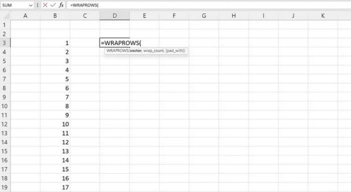
- Add a comma (,) after choosing your numbers’ range.
- Write four for wrap_count. This implies we’ll split the number into four values per row.
- Finish your bracket.
- Enter your keyboard shortcut.
Your final syntax should be as follows.
=WRAPROWS(B3:B22,4)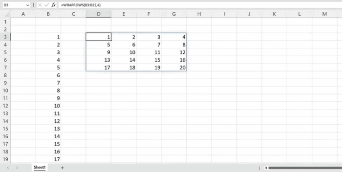
Let’s assume instead that you wish to split it into three values per row. In this case, your syntax will be.
=WRAPROWS(B3:B22,3)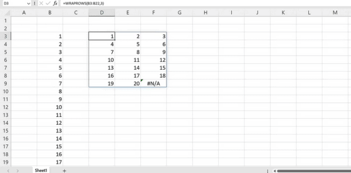
However, as you can see, a #N/A error arises after you have accounted for all the values in your source array. To avoid this, substitute the default value with the padding option. To pad your formula.
- Enter WRAPROWS(.
- Add a comma (,) after choosing your numbers’ range.
- Add a common after you write 3 for wrap_count.
- Enter a space for the pad_with. The symbol symbolizes this “”.
- Enter your keyboard shortcut.
Your final syntax will be as follows.
=WRAPROWS(B3:B22,3," ")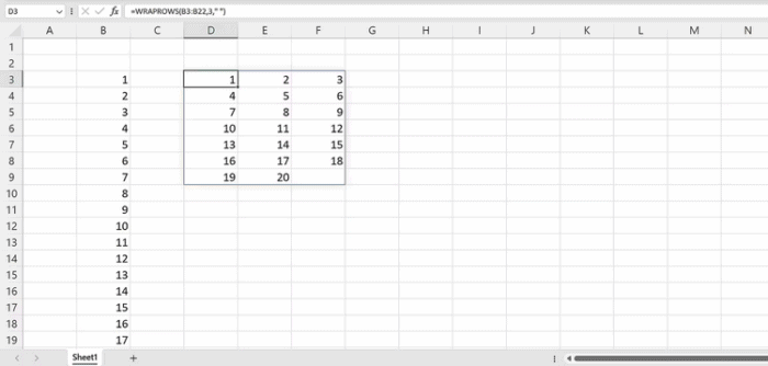
The #N/A errors have been replaced with a space or blank value. That is padding. You may pad with whatever value you like.
WRAPROWS Function Use Case
Consider the following scenario. Assume your table has two columns. Your data table contains a column for students’ names and another for their serial numbers. It would be best if you now split them up into teams as a teacher. You can accomplish this using the WRAPOWS.
- Begin by composing Teams A, B, C, and D.
- Write WRAPROWS( in the cell just under Team A.
- Then, select a data range. This will be the student list.
- Insert a comma.
- Because we wish to split them into four teams, use 4 for the wrap_count.
- Finish your bracket.
- Enter your keyboard shortcut.
While the WRAPROWS formula is excellent for organizing data, there are times when it does not function correctly, just like any other Excel formula. This occurs when the data range is not a one-dimensional array or range. In this case, the WRAPROWS will return a #VALUE! Error.
Consider The Following:
Conclusion:
The WRAPROWS function, as simple as it seems, is really powerful in Excel. Understanding its syntax allows you to organize better and handle data flexibly and efficiently that is simple to use.