
There are several ways to modify your data in Microsoft Excel, and once you’ve figured out how to use it, it’s simple to dig straight into making the most of your spreadsheet. But what if your data arrived in a messy, chaotic state? It might be easier if your data is available to use right away. Fortunately, Excel has functions for swiftly reorganizing your data, and one of these tools is the TOROW function.
What’s TOROW Function In Microsoft Excel?
The TOROW Function creates a single row from a provided data set or an array. Moving the data and arranging it into rows manually would be difficult and time-consuming, particularly if you intend to remove blank spaces or errors from your data. This formula enables you to do both tasks at the same time.
A Look Inside Syntax Of The TOROW Function
The TOROW function’s complete syntax is listed below.
=TOROW(array, [ignore], [scan_by_column])The TOROW function accepts three parameters. The array argument indicates which cells should be reordered into a row.
The optional ignore argument allows you to specify whether cells may be skipped (and under what conditions). The ignore argument accepts four criteria: “0” (the default) retains all values. “1” instructs the Function to ignore blank cells, “2” instructs the Function to ignore cells containing errors (for example, “#NAME!” or “#VALUE!”), and “3” instructs the Function to ignore blank cells and errors.
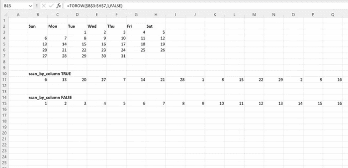
The optional scan_by_column argument instructs Excel on how to construct the row. If this argument is included and set to TRUE, the Function will add the values vertically, column per column. TOROW will add values in horizontal order, row by row, if the argument is set to false or is not included in the Function.
Here’s an example of the difference represented by an array of calendar days. The blank cells at the beginning and end of the array have been disregarded for clarity.
While any functions that are part of the array will be carried over into the new row, it’s a good idea to check and ensure they are displaying as you intend, whether it’s one of the basic Excel functions or a complex LAMBDA formula with multiple arguments and references.
Using TOROW Function In Microsoft Excel
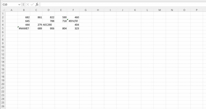
The following is a list of all we can do to help you. It’s primarily numbers; however, there are some blanks and errors to clean up and remove.
To turn this array into a row, click on cell B8, then type the formula below into the cell or the formula bar and hit Enter.
=TOROW(B2:F5)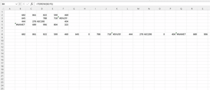
We can see that our array has been turned into a row, but the errors remain. The original array’s blanks have been filled up with zeroes. However, we can tweak the formula to remove such difficulties.
Click cell B11, then type the formula below into the cell or the formula bar and hit Enter.
=TOROW(B2:F5,3)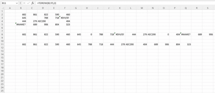
This is the same formula as the one before in B8, but it includes the “ignore” argument, set to “3”, and “ignore blanks and errors,” to remove such elements from our new data set. The one remaining alphanumeric item isn’t a mistake; it only helps demonstrate that this formula works with text and integer values.
Also, Take A Look At:
Conclusion:
When working with Excel, cleaning up untidy data is an unexpected hurdle to productivity. But it doesn’t have to be that way with features like the TOROW function. You can quickly restructure your data to make it clearer and more manageable without slowing you down or diverting your attention from other things. There are plenty of additional ways to learn how to use Microsoft Excel’s strong tools to supercharge your spreadsheets.