
Several functions in Microsoft Excel help you organize your numbers and data. The WRAPCOLS function is one of these functions. This function provides Excel users with a novel and fascinating approach to instantly transform a column into a 2D array, increasing readability and the appearance of data. This post will review the WRAPCOLS function, its features, and how to use it successfully.
What’s WRAPCOLS Function In Excel?
The WRAPCOLS function creates a two-dimensional column array by wrapping the values of rows and columns. Within the formula, you will set the length of each column. This is a dynamic array function and one of the more recent Excel functions. All Microsoft 365 members can access it, even those on the Microsoft 365 Basic plan.
WRAPCOLS Function Syntax In Excel
The WRAPCOLS function’s syntax includes the following parameters.
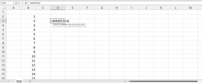
=WRAPCOLS(vector, wrap_count, [pad_with])Let’s go through each function argument.
- The vector represents the reference or cell range to be wrapped.
- The maximum number of values assigned to each column is the wrap_count.
- pad_with is the value you wish to use to pad the row. If no value is supplied, the default in Excel is #N/A.
How To Use WRAPCOLS Function In Excel?
We need example data to get started. To obtain a list of numbers from 1 to 20, use one of the several methods to number rows in Excel. You may use the WRAPCOLS functions to wrap these numbers into a 2D array.
- =WRAPCOLS( Enter your formula in a cell or your formula bar.
- Write a comma after selecting the collection of numbers.
- Write the number five for the wrap_count argument. The number will be split into five columns, each with five values.
- Close the bracket.
- Enter your keyboard shortcut.
Your final syntax will be as follows.
=WRAPCOLS(B2:B21,5)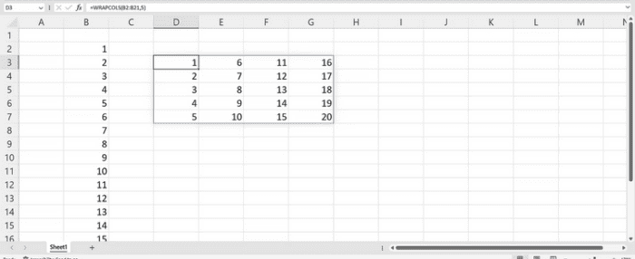
How To Use pad_with Argument In WRAPCOLS Function?
Excel shows a #N/A error by default if the number of values is exhausted and does not equal the number set in the wrap_count. What does it imply? In your first formula, swap out the 4 for a 7. That implies that your syntax should be.
=WRAPCOLS(B2:B21,7)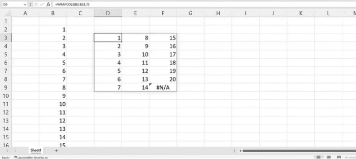
The #N/A an error displays signifies that all values from your source have been considered. To prevent that mistake, supply a value for the pad_with argument.
- Enter WRAPROWS(.
- Add a comma after choosing your range of numbers.
- For the wrap_count argument, enter 7.
- Insert a comma.
- Write a ” ” for the pad_with argument. This means more room!
- Enter your keyboard shortcut.
Your final syntax will be as follows.
=WRAPCOLS(B2:B21,7," ")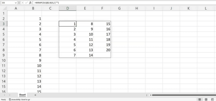
WRAPCOLS Function Use Case
Consider the following scenario. Assume you have a list of dates that you wish to split into quarters. The WRAPCOLS function may be used. All you have to do is.
- Make the function.
- Choose your range. These are the dates.
- Choose 3 for your wrap_count argument.
- As the pad_with argument, you may add a space or even a dash.
- Finally, hit the Enter key on the keyboard.
Your final syntax will be as follows.
=WRAPCOLS(C2:N2,3)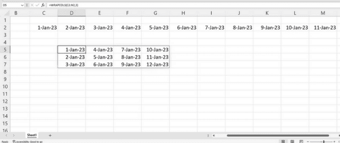
Also, Check:
Conclusion:
In Excel, you can wrap and organize your data into columns regardless of how inconsistent it is. Input the desired number of values in each column and click enter. Aside from this function, you can also use the WRAPROWS function to wrap your data into rows and enjoy the same ease of use.